20. Appendix: Getting Started with Jupyter Notebooks (JupyterLab and Google Colab)#
1. Introduction to Jupyter Notebooks#
Jupyter Notebooks are interactive computing environments that allow you to create and share documents containing live code, equations, visualizations, and narrative text. They have become the standard tool for data science, research, and educational purposes.
1.1 Key Features:#
Interactive Computing: Execute code cells individually and see results immediately
Rich Media Support: Include text, images, graphs, and mathematical equations
Multiple Languages: Support for Python, R, Julia, Scala, and many others
Shareable: Easy to share with colleagues and the broader community
Reproducible: Others can run your notebooks and get the same results
1.2 Common Use Cases:#
Data analysis and visualization
Machine learning experiments
Educational materials and tutorials
Rapid prototyping
Scientific computing and research
1.3 Examples#
# Let's start with a simple example
print("Welcome to Jupyter Notebooks!")
print("This is a Python code cell.")

# You can execute mathematical operations
result = 2 + 2
print(f"2 + 2 = {result}")
Welcome to Jupyter Notebooks!
This is a Python code cell.
2 + 2 = 4
# Import common libraries used in data science
import numpy as np
import pandas as pd
import matplotlib.pyplot as plt

# Create a simple dataset
data = np.random.randn(100)
print(f"Generated {len(data)} random numbers")
print(f"Mean: {np.mean(data):.2f}")
print(f"Standard deviation: {np.std(data):.2f}")
Generated 100 random numbers
Mean: -0.07
Standard deviation: 1.01
2. Getting Started with Google Colab#
Google Colab (Colaboratory) is a free cloud-based Jupyter notebook environment that requires no setup and runs entirely in the browser.
2.1 Advantages of Google Colab:#
No Installation Required: Runs in your web browser
Free GPU/TPU Access: Hardware acceleration for machine learning
Pre-installed Libraries: Most popular data science libraries are already installed
Google Drive Integration: Easy file storage and sharing
Collaboration Features: Real-time collaboration like Google Docs
2.2 Getting Started with Colab:#
Access Google Colab:
Sign in with your Google account
Create a New Notebook:
Click “New notebook” or “File” → “New notebook”
Your notebook will be automatically saved to Google Drive
Basic Operations: check if we’re running in Colab
# This cell demonstrates basic Colab functionality
import sys
print(f"Python version: {sys.version}")

# Check if we're running in Colab
try:
    import google.colab
    print("Running in Google Colab")
    IN_COLAB = True
except ImportError:
    print("Not running in Google Colab")
    IN_COLAB = False
Python version: 3.12.6 (tags/v3.12.6:a4a2d2b, Sep  6 2024, 20:11:23) [MSC v.1940 64 bit (AMD64)]
Not running in Google Colab
Installing Additional Packages in Colab:
# Install packages not included by default
# Use ! to run shell commands
!pip install seaborn plotly

# Import the newly installed packages
import seaborn as sns
import plotly.express as px
print("Additional packages installed successfully!")
Additional packages installed successfully!
WARNING: Ignoring invalid distribution ~upyterlab (C:\Python312\Lib\site-packages)
WARNING: Ignoring invalid distribution ~upyterlab (C:\Python312\Lib\site-packages)
WARNING: Ignoring invalid distribution ~upyterlab (C:\Python312\Lib\site-packages)
Requirement already satisfied: seaborn in c:\python312\lib\site-packages (0.13.2)
Requirement already satisfied: plotly in c:\python312\lib\site-packages (6.2.0)
Requirement already satisfied: numpy!=1.24.0,>=1.20 in c:\python312\lib\site-packages (from seaborn) (2.3.1)
Requirement already satisfied: pandas>=1.2 in c:\python312\lib\site-packages (from seaborn) (2.3.1)
Requirement already satisfied: matplotlib!=3.6.1,>=3.4 in c:\python312\lib\site-packages (from seaborn) (3.10.3)
Requirement already satisfied: narwhals>=1.15.1 in c:\python312\lib\site-packages (from plotly) (1.47.1)
Requirement already satisfied: packaging in c:\python312\lib\site-packages (from plotly) (24.2)
Requirement already satisfied: contourpy>=1.0.1 in c:\python312\lib\site-packages (from matplotlib!=3.6.1,>=3.4->seaborn) (1.3.2)
Requirement already satisfied: cycler>=0.10 in c:\python312\lib\site-packages (from matplotlib!=3.6.1,>=3.4->seaborn) (0.12.1)
Requirement already satisfied: fonttools>=4.22.0 in c:\python312\lib\site-packages (from matplotlib!=3.6.1,>=3.4->seaborn) (4.58.5)
Requirement already satisfied: kiwisolver>=1.3.1 in c:\python312\lib\site-packages (from matplotlib!=3.6.1,>=3.4->seaborn) (1.4.8)
Requirement already satisfied: pillow>=8 in c:\python312\lib\site-packages (from matplotlib!=3.6.1,>=3.4->seaborn) (11.3.0)
Requirement already satisfied: pyparsing>=2.3.1 in c:\python312\lib\site-packages (from matplotlib!=3.6.1,>=3.4->seaborn) (3.2.3)
Requirement already satisfied: python-dateutil>=2.7 in c:\python312\lib\site-packages (from matplotlib!=3.6.1,>=3.4->seaborn) (2.9.0.post0)
Requirement already satisfied: pytz>=2020.1 in c:\python312\lib\site-packages (from pandas>=1.2->seaborn) (2025.2)
Requirement already satisfied: tzdata>=2022.7 in c:\python312\lib\site-packages (from pandas>=1.2->seaborn) (2025.2)
Requirement already satisfied: six>=1.5 in c:\python312\lib\site-packages (from python-dateutil>=2.7->matplotlib!=3.6.1,>=3.4->seaborn) (1.17.0)
Mounting Google Drive in Colab:
# Mount Google Drive to access your files
if IN_COLAB:
    from google.colab import drive
    drive.mount('/content/drive')
    print("Google Drive mounted successfully!")

    # You can now access files in your Google Drive
    # Files will be available at /content/drive/MyDrive/
    # You may open a terminal and use it to display the list of folders and files in your Google Drive.
    # This can help verify that your files are correctly uploaded and accessible from the environment.
3. Setting Up JupyterLab#
JupyterLab is the next-generation web-based user interface for the Jupyter Project. It provides a more powerful and flexible environment than the classic Jupyter Notebook.
3.1 Installing JupyterLab#
The preferred way to install JupyterLab is by using pip.
# Install JupyterLab using pip
pip install jupyterlab

# Launch JupyterLab
jupyter lab
3.2 Launch JupyterLab#
To launch JupyterLab, open a command prompt or terminal, navigate to your target folder, and enter the following command:
# Launch JupyterLab
jupyter lab
3.3 JupyterLab Features#
JupyterLab provides enhanced features over classic Jupyter:
Flexible user interface
Multiple document support
File browser integrationTerminal integration
Extension system
Drag and drop functionality
Multiple kernels support
3.4 JupyterLab Extensions#
JupyterLab extensions can be installed via pip. Below are some popular JupyterLab extensions:
Variable Inspector: Shows variables in the current namespace
Table of Contents: Generates TOC of contents from notebook headers
Git: Git integration for version control
Plotly: Enhanced support for Plotly visualizations
Spreadsheet: Provides Excel-like spreadsheet functionality
3.5 Customizing JupyterLab#
You can customize JupyterLab through the Settings menu or by editing configuration files directly. Common customizations include:
Theme selection (dark/light)
Keyboard shortcuts
Extension management
Notebook cell execution settings
File browser preferences
These settings allow users to tailor the JupyterLab environment to their workflow and preferences.
4. Google Colab vs JupyterLab#
4.1 Comparing Google Colab vs JupyterLab#
Here’s a detailed comparison between Google Colab and JupyterLab across various dimensions:
Feature |
Google Colab |
JupyterLab |
|---|---|---|
Cost |
Free (with usage limits) |
Free (self-hosted) |
Setup Required |
None - runs in browser |
Installation required |
Hardware Access |
Free GPU/TPU access |
Local hardware only |
Storage |
Google Drive integration |
Local file system |
Collaboration |
Real-time collaboration |
Limited collaboration |
Offline Access |
No - requires internet connection |
Yes - fully offline capable |
Customization |
Limited theme options |
Highly customizable |
Library Management |
Pre-installed common libraries |
Full control over environment |
Performance |
High-performance cloud hardware |
Depends on local hardware |
Data Privacy |
Data stored on Google servers |
Full control over data |
Session Persistence |
Sessions timeout (12-24 hours) |
Persistent sessions |
File Management |
Google Drive interface |
Full file system access |
Debugging Tools |
Basic debugging features |
Advanced debugging |
Version Control |
Basic Git support |
Full Git integration |
Multi-language Support |
Python focus |
Python, R, Julia, Scala |
4.2 When to Use Google Colab#
Choose Google Colab when:
Getting started with data science or machine learning
You need free GPU or TPU access
You are working on small to medium projects
Collaboration is important
You don’t want to manage a local environment
You use it occasionally or for learning purposes
You need to share your work easily
4.3 When to Use JupyterLab#
Choose JupyterLab when:
You are working with sensitive or proprietary data
You need offline access
You require specific software versions
You are working with large datasets
You need extensive customization
You are in a professional or enterprise environment
You want full control over the environment
You are working with multiple programming languages
5. Installing and Managing Libraries#
One of the most important aspects of working with Jupyter notebooks is managing libraries and packages. The approach differs between Google Colab and JupyterLab.
5.1 Understanding Package Management Systems#
First, let’s understand the different package managers:
import sys
print(f"Python version: {sys.version}")
print(f"Python executable: {sys.executable}")

# Check which package managers are available
import subprocess
import os

def check_package_manager(command):
    try:
        result = subprocess.run([command, '--version'],
                              capture_output=True, text=True, timeout=5)
        return result.returncode == 0
    except:
        return False

managers = {
    'pip': check_package_manager('pip'),
    'conda': check_package_manager('conda'),
    'mamba': check_package_manager('mamba')
}

print("\nAvailable package managers:")
for manager, available in managers.items():
    status = "✓ Available" if available else "✗ Not available"
    print(f"  {manager}: {status}")
Python version: 3.12.6 (tags/v3.12.6:a4a2d2b, Sep  6 2024, 20:11:23) [MSC v.1940 64 bit (AMD64)]
Python executable: C:\Python312\python.exe

Available package managers:
  pip: ✓ Available
  conda: ✗ Not available
  mamba: ✗ Not available
5.2 Installing Libraries in Google Colab#
This code demonstrates six common ways to install Python libraries in a Google Colab environment using pip:
# Method 1: Using pip (most common in Colab)
# The ! prefix runs shell commands
!pip install seaborn plotly scikit-learn

# Method 2: Installing specific versions
!pip install pandas==1.5.3 numpy>=1.20.0

# Method 3: Installing from requirements file
# First, create a requirements.txt file
requirements_content = """
matplotlib>=3.5.0
seaborn>=0.11.0
plotly>=5.0.0
scikit-learn>=1.0.0
requests>=2.25.0
"""

# Write to file (in Colab)
with open('requirements.txt', 'w') as f:
    f.write(requirements_content)

# Install from requirements file
!pip install -r requirements.txt

print("Libraries installed successfully in Colab!")

# Method 4: Installing from GitHub repositories
!pip install git+https://github.com/user/repository.git

# Method 5: Installing with specific options
!pip install --upgrade tensorflow  # Upgrade existing package
!pip install --no-cache-dir torch   # Install without using cache
!pip install --user package_name    # Install for current user only

# Method 6: Installing development versions
!pip install --pre scikit-learn  # Install pre-release version
5.3 Checking Installed Libraries in Google Colab#
This code demonstrates different ways to check the installation status of Python packages in a Google Colab environment:
Using pip list with grep: Filters and displays installed packages matching pandas, numpy, or matplotlib.
Using pip show: Retrieves detailed metadata (version, location, dependencies) for the pandas package.
Programmatic Check: Defines a function to check if a given package is installed using import. It then loops through a list of common libraries (pandas, numpy, matplotlib, seaborn, plotly) and prints whether each is installed.
# Checking installed packages in Colab
!pip list | grep -E "(pandas|numpy|matplotlib)"

# Get detailed information about a package
!pip show pandas

# Check if a package is installed programmatically
def check_package_installed(package_name):
    try:
        __import__(package_name)
        return True
    except ImportError:
        return False

packages_to_check = ['pandas', 'numpy', 'matplotlib', 'seaborn', 'plotly']
print("Package installation status:")
for package in packages_to_check:
    status = "✓ Installed" if check_package_installed(package) else "✗ Not installed"
    print(f"  {package}: {status}")
5.4 Installing Libraries in JupyterLab#
This code outlines multiple methods for installing Python packages in a JupyterLab environment, with a focus on ensuring the packages are installed into the correct Python environment:
# Method 1: Using pip from within notebook
import sys
!{sys.executable} -m pip install seaborn plotly scikit-learn

# This ensures pip installs to the same Python environment as the notebook

# Method 2: Using conda (if available)
# Note: This works if JupyterLab is running in a conda environment
!conda install -c conda-forge seaborn plotly scikit-learn -y

# Method 3: Using mamba (faster conda alternative)
!mamba install -c conda-forge seaborn plotly scikit-learn -y

# Method 4: Installing in the correct environment
# This is crucial when you have multiple Python environments

# Check current environment
import os
print(f"Current Python executable: {sys.executable}")
print(f"Current working directory: {os.getcwd()}")

# Install to current environment
!{sys.executable} -m pip install --user package_name
5.5 Managing Virtual Environments#
a virtual environment is an isolated Python workspace that allows you to install and manage packages separately from the system-wide Python installation. Using a virtual environment ensures that:
Projects do not interfere with each other’s dependencies.
You can safely test or upgrade packages without breaking other work.
Your Jupyter Notebook or Colab environment remains clean and reproducible.
This code introduces virtual environment best practices and demonstrates how to create and inspect a requirements.txt file in a Python or Jupyter environment:
# Understanding virtual environments
print("Virtual Environment Best Practices:")
print("1. Create separate environments for different projects")
print("2. Use requirements.txt to track dependencies")
print("3. Activate the correct environment before starting Jupyter")

# Example of creating a requirements.txt from current environment
!pip freeze > requirements.txt

# Read and display the requirements
try:
    with open('requirements.txt', 'r') as f:
        requirements = f.read()
    print("\nCurrent environment requirements:")
    print(requirements[:500] + "..." if len(requirements) > 500 else requirements)
except FileNotFoundError:
    print("No requirements.txt file found")
Virtual Environment Best Practices:
1. Create separate environments for different projects
2. Use requirements.txt to track dependencies
3. Activate the correct environment before starting Jupyter

Current environment requirements:
annotated-types==0.7.0
anyio==3.7.1
argon2-cffi==23.1.0
argon2-cffi-bindings==21.2.0
arrow==1.3.0
asttokens==3.0.0
async-lru==2.0.4
attrs==24.3.0
babel==2.16.0
beautifulsoup4==4.12.3
bleach==6.2.0
blinker==1.8.2
certifi==2024.12.14
cffi==1.17.1
charset-normalizer==3.4.0
click==8.1.7
colorama==0.4.6
comm==0.2.2
contourpy==1.3.2
cycler==0.12.1
debugpy==1.8.11
decorator==5.1.1
defusedxml==0.7.1
executing==2.1.0
fastapi==0.104.1
fastjsonschema==2.21.1
Flask==2.3.3
Flask-Cors==4.0.0
fonttools==4.58.5...
WARNING: Ignoring invalid distribution ~upyterlab (C:\Python312\Lib\site-packages)
6. Basic Operations and Examples#
Let’s explore basic operations that work in both environments:
6.1 Working with Data#
This code generates and displays a sample time-series dataset using NumPy and pandas, commonly used for data analysis or visualization practice.
# Create sample data
import numpy as np
import pandas as pd
import matplotlib.pyplot as plt

# Generate sample dataset
np.random.seed(42)
dates = pd.date_range('2023-01-01', periods=100, freq='D')
values = np.cumsum(np.random.randn(100)) + 100

df = pd.DataFrame({
    'date': dates,
    'value': values,
    'category': np.random.choice(['A', 'B', 'C'], 100)
})

print("Sample Dataset:")
print(df.head())
print(f"\nDataset shape: {df.shape}")
Sample Dataset:
        date       value category
0 2023-01-01  100.496714        A
1 2023-01-02  100.358450        B
2 2023-01-03  101.006138        A
3 2023-01-04  102.529168        A
4 2023-01-05  102.295015        C

Dataset shape: (100, 3)
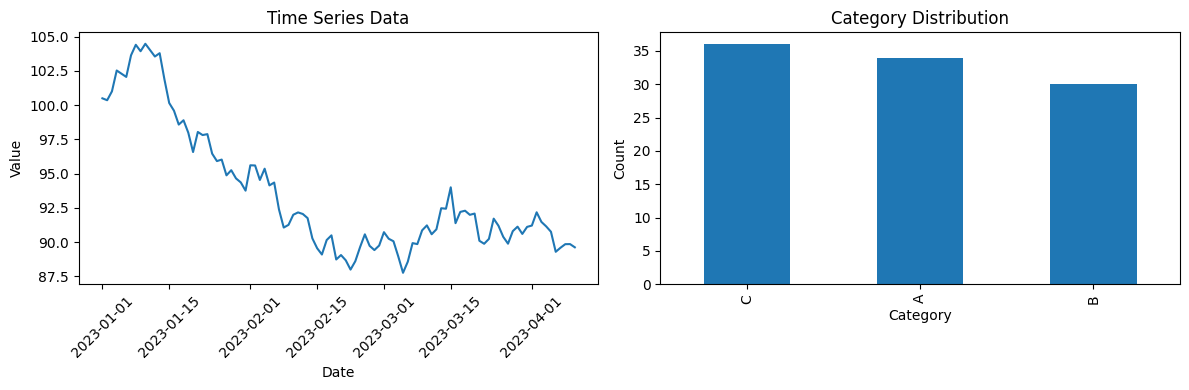
6.2 Data Visualization#
This code generates two side-by-side visualizations using matplotlib to explore a sample dataset (df), providing insights into time series trends and categorical distribution.
# Create visualizations
plt.figure(figsize=(12, 4))

# Time series plot
plt.subplot(1, 2, 1)
plt.plot(df['date'], df['value'])
plt.title('Time Series Data')
plt.xlabel('Date')
plt.ylabel('Value')
plt.xticks(rotation=45)

# Category distribution
plt.subplot(1, 2, 2)
df['category'].value_counts().plot(kind='bar')
plt.title('Category Distribution')
plt.xlabel('Category')
plt.ylabel('Count')

plt.tight_layout()
plt.show()
6.3 Statistical Analysis#
This code performs basic statistical analysis on the df DataFrame, summarizing the numerical column ‘value’ and exploring category-based differences.
# Basic statistical analysis
print("Statistical Summary:")
print(df['value'].describe())

# Convert dates to numeric format for correlation
date_numeric = df['date'].map(pd.Timestamp.toordinal)
correlation = date_numeric.corr(df['value'])
print(f"\nCorrelation between date and value: {correlation:.3f}")

# Group by category
category_stats = df.groupby('category')['value'].agg(['mean', 'std', 'count'])
print("\nStatistics by Category:")
print(category_stats)
Statistical Summary:
count    100.000000
mean      93.594818
std        4.643998
min       87.753344
25%       90.132492
50%       91.727866
75%       95.940029
max      104.480611
Name: value, dtype: float64

Correlation between date and value: -0.800

Statistics by Category:
               mean       std  count
category
A         93.933355  5.040641     34
B         94.168522  4.683877     30
C         92.797001  4.221481     36
6.4 Working with External Data#
This code explains common methods to load external data into a Python environment (JupyterLab or Google Colab) and demonstrates loading a sample dataset from a public URL.
# Example of reading data from different sources
# Note: This would work differently in Colab vs JupyterLab

print("Methods to load external data:")
print("1. Local files (JupyterLab): pd.read_csv('local_file.csv')")
print("2. Google Drive (Colab): pd.read_csv('/content/drive/MyDrive/file.csv')")
print("3. URLs (both): pd.read_csv('https://example.com/data.csv')")
print("4. APIs (both): Using requests library")

# Example with a public dataset
try:
    # This URL provides sample data
    url = "https://raw.githubusercontent.com/mwaskom/seaborn-data/master/iris.csv"
    iris_df = pd.read_csv(url)
    print(f"\nLoaded Iris dataset: {iris_df.shape}")
    print(iris_df.head())
except Exception as e:
    print(f"Could not load external data: {e}")
Methods to load external data:
1. Local files (JupyterLab): pd.read_csv('local_file.csv')
2. Google Drive (Colab): pd.read_csv('/content/drive/MyDrive/file.csv')
3. URLs (both): pd.read_csv('https://example.com/data.csv')
4. APIs (both): Using requests library

Loaded Iris dataset: (150, 5)
   sepal_length  sepal_width  petal_length  petal_width species
0           5.1          3.5           1.4          0.2  setosa
1           4.9          3.0           1.4          0.2  setosa
2           4.7          3.2           1.3          0.2  setosa
3           4.6          3.1           1.5          0.2  setosa
4           5.0          3.6           1.4          0.2  setosa